Planning follows a straight path
Place cells in the hippocampus fire when an animal is at a particular place. Instead of asking what a single cell does, take the whole population at position  as one vector,
 , where
 sets the spatial scale.The scale grows like
 , which mirrors the dorsoventral axis of the hippocampus. We ask one thing of this vector: its inner products should be the transition probabilities of a random walk,
 (1)
where  is the probability of reaching
 from in steps, normalized so that
 . If the elements of
 are also required to be non-negative, each one becomes a localized place field, and together the fields tile the space.
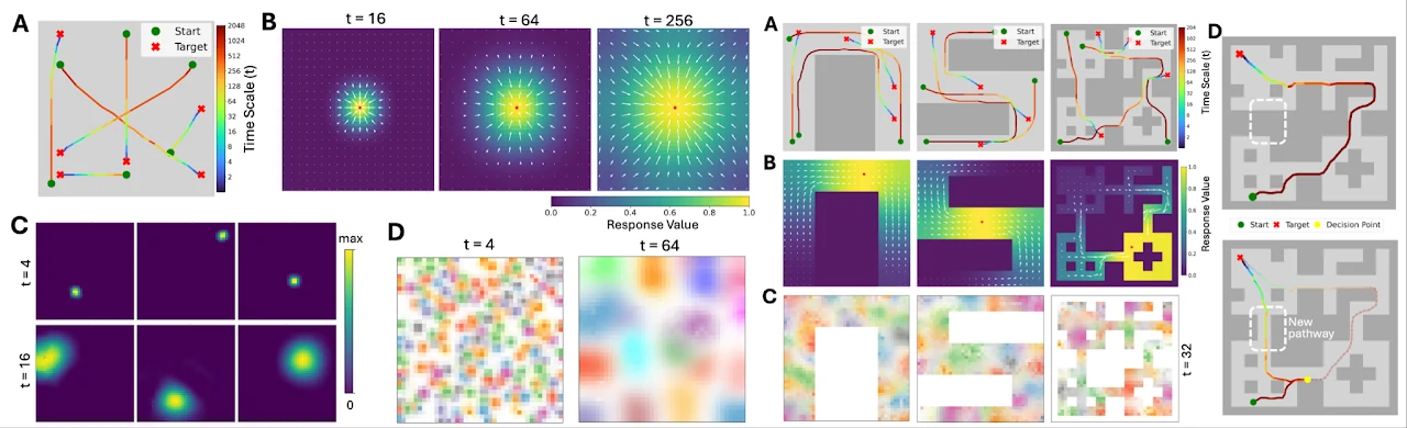
Figure 1. Place fields at several time scales, and the paths planned from them in open fields and mazes.
Why the path is straight
Every has unit norm, so (1) gives
 (2)
Climbing  toward a goal is therefore the same as descending the Euclidean distance to
 . In the maze the route bends around walls. In the embedding it heads straight for the goal.
Many scales
One scale is not enough. Near the goal a small gives a sharp signal, and far from it only a large reaches at all. The scales are tied together by
 (3)
which is the recursion of dynamic programming.No successful trajectory is needed to learn this. The walk is random. At each step the planner uses the scale with the largest gradient.
Video 1. The field for a fixed goal as grows, then the path found by the planner below.
# Setup omitted: A is the adjacency matrix of the free cells of the maze,
# deg its row sums, and P = I/2 + A/(2 deg) the lazy random walk on them.

def q(Pt):
    """Normalized transition probability, so that q(x | x, t) = 1."""
    K = Pt / deg[None, :]        # symmetric kernel of the reversible walk
    d = np.sqrt(np.diag(K))
    return K / np.outer(d, d)

# Scales t = 1, 2, 4, ...: P_2t = P_t squared.
scales, Pt = [], P.copy()
for k in range(12):
    scales.append(q(Pt))
    Pt = Pt @ Pt

def plan(x, y):
    """Greedy ascent on q(y | x, t), at the scale with the largest gain."""
    path = [x]
    while x != y:
        nbrs = np.nonzero(A[x])[0]
        gain = np.array([[Q[n, y] - Q[x, y] for n in nbrs] for Q in scales])
        x = nbrs[gain.max(0).argmax()]
        path.append(x)
return path| symbol | meaning |
|---|---|
 | positions |
| number of steps of the walk |
| population vector of place cells |
| normalized transition probability |
Table 1. Notation.
Reference
- M. Zhao, D. Xu, D. Kong, W.-H. Zhang, Y. N. Wu. Place Cells as Multi-Scale Position Embeddings: Random Walk Transition Kernels for Path Planning. NeurIPS 2025.